by Ehtsham Elahi
with James McInerney, Nathan Kallus, Dario Garcia Garcia and Justin Basilico
Introduction
This writeup is well-nigh using reinforcement learning to construct an optimal list of recommendations when the user has a finite time upkeep to make a visualization from the list of recommendations. Working within the time upkeep introduces an uneaten resource constraint for the recommender system. It is similar to many other visualization problems (for e.g. in economics and operations research) where the entity making the visualization has to find tradeoffs in the squatter of finite resources and multiple (possibly conflicting) objectives. Although time is the most important and finite resource, we think that it is an often ignored speciality of recommendation problems.
In wing to relevance of the recommendations, time upkeep moreover determines whether users will winnow a recommendation or welsh their search. Consider the scenario that a user comes to the Netflix homepage looking for something to watch. The Netflix homepage provides a large number of recommendations and the user has to evaluate them to segregate what to play. The evaluation process may include trying to recognize the show from its box art, watching trailers, reading its synopsis or in some cases reading reviews for the show on some external website. This evaluation process incurs a forfeit that can be measured in units of time. Variegated shows will require variegated amounts of evaluation time. If it’s a popular show like Stranger Things then the user may once be enlightened of it and may incur very little forfeit surpassing choosing to play it. Given the limited time budget, the recommendation model should construct a slate of recommendations by considering both the relevance of the items to the user and their evaluation cost. Balancing both of these aspects can be difficult as a highly relevant item may have a much higher evaluation forfeit and it may not fit within the user’s time budget. Having a successful slate therefore depends on the user’s time budget, relevance of each item as well as their evaluation cost. The goal for the recommendation algorithm therefore is to construct slates that have a higher endangerment of engagement from the user with a finite time budget. It is important to point out that the user’s time budget, like their preferences, may not be directly observable and the recommender system may have to learn that in wing to the user’s latent preferences.
A typical slate recommender system
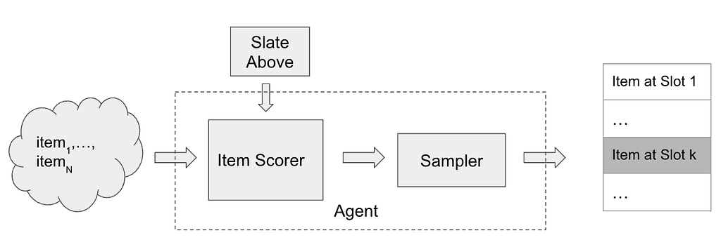
We are interested in settings where the user is presented with a slate of recommendations. Many recommender systems rely on a thief style tideway to slate construction. A thief recommender system constructing a slate of K items may squint like the following:
To insert an element at slot k in the slate, the item scorer scores all of the misogynist N items and may make use of the slate synthetic so far (slate above) as spare context. The scores are then passed through a sampler (e.g. Epsilon-Greedy) to select an item from the misogynist items. The item scorer and the sampling step are the main components of the recommender system.
Problem formulation
Let’s make the problem of upkeep constrained recommendations increasingly touchable by considering the pursuit (simplified) setting. The recommender system presents a one dimensional slate (a list) of K items and the user examines the slate sequentially from top to bottom.
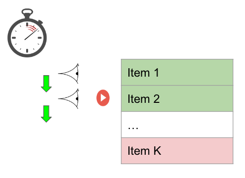
The user has a time upkeep which is some positive real valued number. Let’s seem that each item has two features, relevance (a scalar, higher value of relevance ways that the item is increasingly relevant) and forfeit (measured in a unit of time). Evaluating each recommendation consumes from the user’s time upkeep and the user can no longer scan the slate once the time upkeep has exhausted. For each item examined, the user makes a probabilistic visualization to slosh the recommendation by flipping a forge with probability of success proportional to the relevance of the video. Since we want to model the user’s probability of consumption using the relevance feature, it is helpful to think of relevance as a probability directly (between 0 and 1). Unmistakably the probability to segregate something from the slate of recommendations is dependent not only on the relevance of the items but moreover on the number of items the user is worldly-wise to examine. A recommendation system trying to maximize the user’s engagement with the slate needs to pack in as many relevant items as possible within the user budget, by making a trade-off between relevance and cost.
Connection with the 0/1 Knapsack problem
Let’s squint at it from flipside perspective. Consider the pursuit definitions for the slate recommendation problem described above
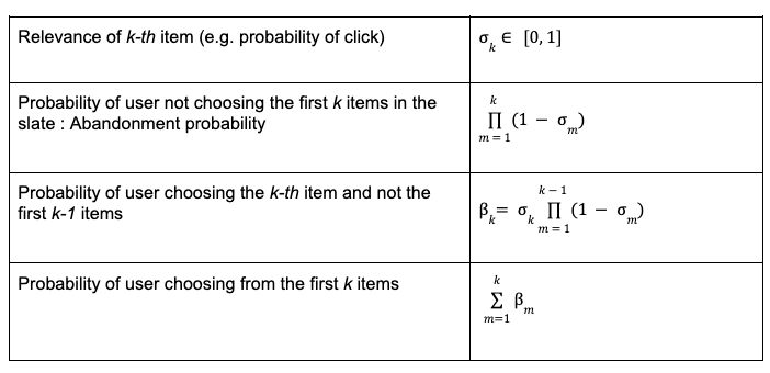
Clearly the zealotry probability is small if the items are highly relevant (high relevance) or the list is long (since the zealotry probability is a product of probabilities). The zealotry option is sometimes referred to as the null choice/arm in thief literature.
This problem has well-spoken connections with the 0/1 Knapsack problem in theoretical computer science. The goal is to find the subset of items with the highest total utility such that the total forfeit of the subset is not greater than the user budget. If β_i and c_i are the utility and forfeit of the i-th item and u is the user budget, then the upkeep constrained recommendations can be formulated as
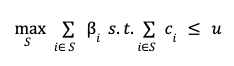
There is an spare requirement that optimal subset S be sorted in descending order equal to the relevance of items in the subset.
The 0/1 Knapsack problem is a well studied problem and is known to be NP-Complete. There are many injudicious solutions to the 0/1 Knapsack problem. In this writeup, we propose to model the upkeep constrained recommendation problem as a Markov Visualization process and use algorithms from reinforcement learning (RL) to find a solution. It will wilt well-spoken that the RL based solution to upkeep constrained recommendation problems fits well within the recommender system tracery for slate construction. To begin, we first model the upkeep constrained recommendation problem as a Markov Decision Process.
Budget constrained recommendations as a Markov Decision Process
In a Markov visualization process, the key component is the state incubation of the environment as a function of the current state and the whoopee taken by the agent. In the MDP formulation of this problem, the wage-earner is the recommender system and the environment is the user interacting with the recommender system. The wage-earner constructs a slate of K items by repeatedly selecting deportment it deems towardly at each slot in the slate. The state of the environment/user is characterized by the misogynist time upkeep and the items examined in the slate at a particular step in the slate browsing process. Specifically, the pursuit table defines the Markov Visualization Process for the upkeep constrained recommendation problem,
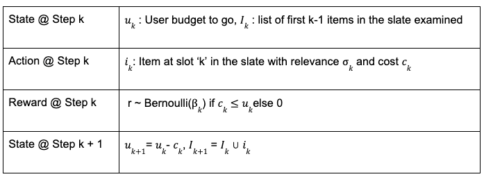
In real world recommender systems, the user upkeep may not be observable. This problem can be solved by computing an estimate of the user upkeep from historical data (e.g. how long the user scrolled surpassing withdrawing in the historical data logs). In this writeup, we seem that the recommender system/agent has wangle to the user upkeep for sake of simplicity.
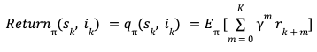
The slate generation task whilom is an episodic task i-e the recommender wage-earner is tasked with choosing K items in the slate. The user provides feedback by choosing one or zero items from the slate. This can be viewed as a binary reward r per item in the slate. Let π be the recommender policy generating the slate and γ be the reward unbelieve factor, we can then pinpoint the discounted return for each state, whoopee pair as,
State, Whoopee Value function estimation
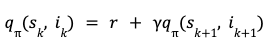
The reinforcement learning algorithm we employ is based on estimating this return using a model. Specifically, we use Temporal Difference learning TD(0) to estimate the value function. Temporal difference learning uses Bellman’s equation to pinpoint the value function of current state and whoopee in terms of value function of future state and action.
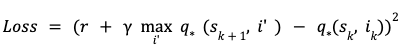
Based on this Bellman’s equation, a squared loss for TD-Learning is,
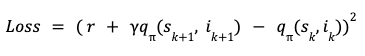
The loss function can be minimized using semi-gradient based methods. Once we have a model for q, we can use that as the item scorer in the whilom slate recommender system architecture. If the unbelieve factor γ =0, the return for each (state, action) pair is simply the firsthand user feedback r. Therefore q with γ = 0 corresponds to an item scorer for a contextual thief wage-earner whereas for γ > 0, the recommender corresponds to a (value function based) RL agent. Therefore simply using the model for the value function as the item scorer in the whilom system tracery makes it very easy to use an RL based solution.
Budget constrained Recommendation Simulation
As in other applications of RL, we find simulations to be a helpful tool for studying this problem. Unelevated we describe the generative process for the simulation data,
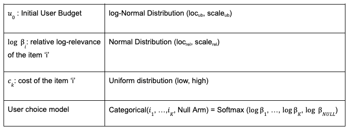
Note that, instead of sampling the per-item Bernoulli, we can alternatively sample once from a well-defined distribution with relative relevances for items and a stock-still weight for the null arm. The whilom generative process for simulated data depends on many hyper-parameters (loc, scale etc.). Each setting of these hyper-parameters results in a variegated simulated dataset and it’s easy to realize many simulated datasets in parallel. For the experiments below, we fix the hyper-parameters for the forfeit and relevance distributions and sweep over the initial user upkeep distribution’s location parameter. The tying notebook contains the word-for-word settings of the hyper-parameters used for the simulations.
Metric
A slate recommendation algorithm generates slates and then the user model is used to predict the success/failure of each slate. Given the simulation data, we can train various recommendation algorithms and compare their performance using a simple metric as the stereotype number of successes of the generated slates (referred to as play-rate below). In wing to play-rate, we squint at the effective-slate-size as well, which we pinpoint to be the number of items in the slate that fit the user’s time budget. As mentioned earlier, one of the ways play-rate can be improved is by constructing larger constructive slates (with relevant items of-course) so looking at this metric helps understand the mechanism of the recommendation algorithms.
On-policy learning results
Given the flexibility of working in the simulation setting, we can learn to construct optimal slates in an on-policy manner. For this, we start with some initial random model for the value function, generate slates from it, get user feedback (using the user model) and then update the value function model using the feedback and alimony repeating this loop until the value function model converges. This is known as the SARSA algorithm.
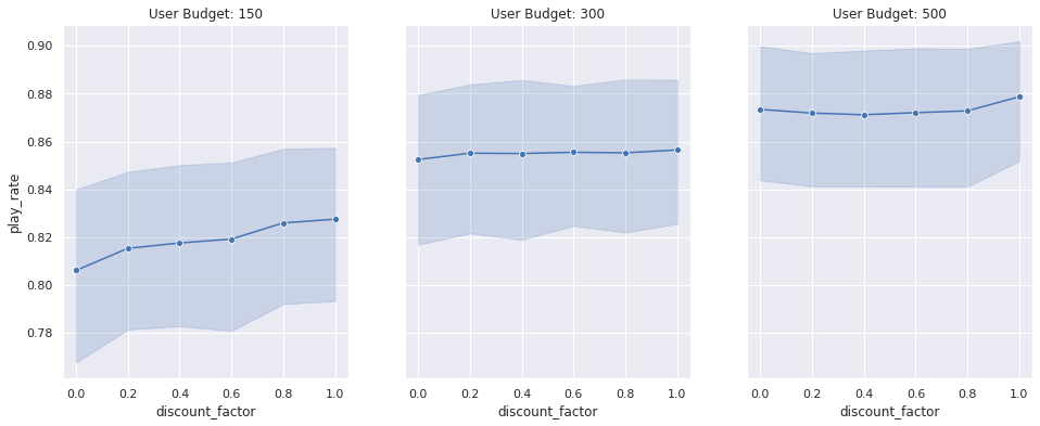
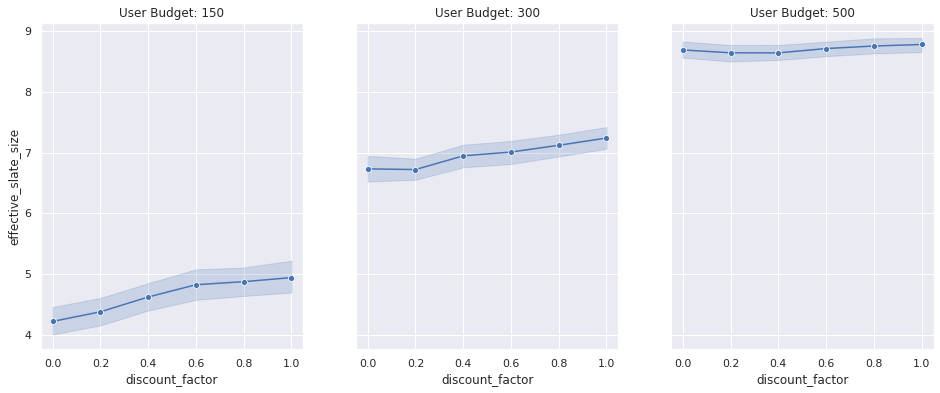
The pursuit set of results show how the learned recommender policies behave in terms of metric of success, play-rate for variegated settings of the user upkeep distributions’s location parameter and the unbelieve factor. In wing to the play rate, we moreover show the constructive slate size, stereotype number of items that fit within the user budget. While the play rate changes are statistically insignificant (the shaded areas are the 95% conviction intervals unscientific using bootstrapping simulations 100 times), we see a well-spoken trend in the increase in the constructive slate size (γ > 0) compared to the contextual thief (γ= 0)
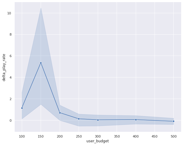
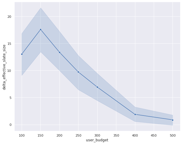
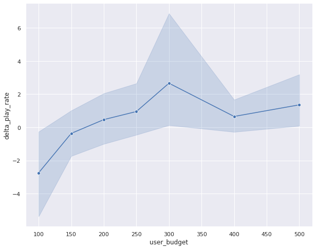
We can unquestionably get a increasingly statistically sensitive result by comparing the result of the contextual thief with an RL model for each simulation setting (similar to a paired comparison in paired t-test). Unelevated we show the transpiration in play rate (delta play rate) between any RL model (shown with γ = 0.8 unelevated as an example) and a contextual thief (γ = 0). We compare the transpiration in this metric for variegated user upkeep distributions. By performing this paired comparison, we see a statistically significant lift in play rate for small to medium upkeep user upkeep ranges. This makes intuitive sense as we would expect both approaches to work equally well when the user upkeep is too large (therefore the item’s forfeit is irrelevant) and the RL algorithm only outperforms the contextual thief when the user upkeep is limited and finding the trade-off between relevance and forfeit is important. The increase in the constructive slate size is plane increasingly dramatic. This result unmistakably shows that the RL wage-earner is performing largest by minimizing the zealotry probability by packing increasingly items within the user budget.
Off-policy learning results
So far the results have shown that in the upkeep constrained setting, reinforcement learning outperforms contextual bandit. These results have been for the on-policy learning setting which is very easy to simulate but difficult to execute in realistic recommender settings. In a realistic recommender, we have data generated by a variegated policy (called a policies policy) and we want to learn a new and largest policy from this data (called the target policy). This is tabbed the off-policy setting. Q-Learning is one well known technique that allows us to learn optimal value function in an off-policy setting. The loss function for Q-Learning is very similar to the TD(0) loss except that it uses Bellman’s optimality equation instead
This loss can then be minimized using semi-gradient techniques. We estimate the optimal value function using Q-Learning and compare its performance with the optimal policy learned using the on-policy SARSA setup. For this, we generate slates using Q-Learning based optimal value function model and compare the play-rate with the slates generated using the optimal policy learned with SARSA. Unelevated is result of the paired comparison between SARSA and Q-Learning,
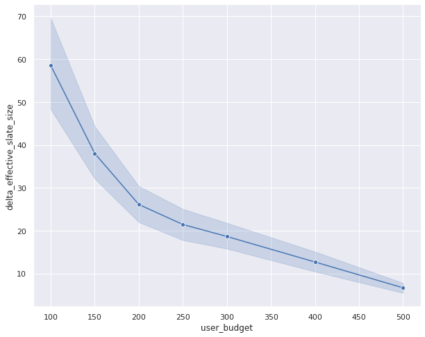
In this result, the transpiration in the play-rate between on-policy and off-policy models is tropical to zero (see the error bars crossing the zero-axis). This is a favorable result as this shows that Q-Learning results in similar performance as the on-policy algorithm. However, the constructive slate size is quite variegated between Q-Learning and SARSA. Q-Learning seems to be generating very large constructive slate sizes without much difference in the play rate. This is an intriguing result and needs a little increasingly investigation to fully uncover. We hope to spend increasingly time understanding this result in future.
Conclusion:
To conclude, in this writeup we presented the upkeep constrained recommendation problem and showed that in order to generate slates with higher chances of success, a recommender system has to wastefulness both the relevance and forfeit of items so that increasingly of the slate fits within the user’s time budget. We showed that the problem of upkeep constrained recommendation can be modeled as a Markov Visualization Process and we can find a solution to optimal slate construction under upkeep constraints using reinforcement learning based methods. We showed that the RL outperforms contextual bandits in this problem setting. Moreover, we compared the performance of On-policy and Off-policy approaches and found the results to be comparable in terms of metrics of success.
Code
Reinforcement Learning for Upkeep Constrained Recommendations was originally published in Netflix TechBlog on Medium, where people are standing the conversation by highlighting and responding to this story.